Introducing the Kernel Heaping Package III
In the second part of this blog series, I showed how to compute spatial kernel density estimates based on area-level data. The Kernelheaping package also supports boundary-corrected kernel density estimation, which allows us to exclude certain areas, where we know that the density must be zero. One example is estimating the population density where we like to exclude uninhabited areas such as lakes, forests, parks etc. The Kernelheaping package employs a boundary correction method, where each single kernel is restricted to the area of interest. We continue with our example of elderly people in Berlin from part two:
library(maptools)
library(dplyr)
library(fields)
library(ggplot2)
library(RColorBrewer)
library(Kernelheaping)
library(rgeos)
library(rgdal)
Again, we load a shapefile with the administrative districts, available from: https://www.statistik-berlin-brandenburg.de/opendata/RBS_OD_LOR_2015_12.zip
data <- read.csv2("EWR201512E_Matrix.csv")
berlin <- readOGR("RBS_OD_LOR_2015_12/RBS_OD_LOR_2015_12.shp")
berlin <- spTransform(berlin, CRS("+proj=longlat +datum=WGS84"))
We load an OpenStreetMap file including shapes or polygons with information on uninhabited areas such as lakes, rivers, forests and parks: https://daten.berlin.de/datensaetze/openstreetmap-daten-für-berlin
berlinN <- readOGR("berlin-latest-free.shp/gis_osm_landuse_a_free_1.shp") # land
berlinWater <- readOGR("berlin-latest-free.shp/gis_osm_water_a_free_1.shp") # water
We specifically exclude residential areas and split the shapefile into the two remaining categories (“Nature” and “Other”):
table(berlinN@data$fclass)

berlinN <- berlinN[!(berlinN@data$fclass == "residential"), ]

berlinGreen <- berlinN[(berlinN@data$fclass %in%
c("forest", "grass", "nature_reserve", "park",
    "cemetery", "allotments", "farm", "meadow",
    "orchard", "vineyard", "heath")), ]

berlinOther <- berlinN[!(berlinN@data$fclass %in%
c("forest", "grass", "nature_reserve", "park",
  "cemetery", "allotments", "farm", "meadow",
  "orchard", "vineyard", "heath")), ]
These shapes are very complicated with many polygons. Thus we simplify them with the gSimplify() function from the rgeos package:
berlinGreen <- spTransform(gSimplify(berlinGreen, tol = 0.0005, topologyPreserve = FALSE),
                   CRS("+proj=longlat +datum=WGS84"))

berlinOther <- spTransform(gSimplify(berlinOther, tol = 0.0005, topologyPreserve = FALSE),
                           CRS("+proj=longlat +datum=WGS84"))

berlinWater <- spTransform(gSimplify(berlinWater, tol = 0.0005, topologyPreserve = FALSE),
                           CRS("+proj=longlat +datum=WGS84"))
For the dshapebivr() and dshapebivrProp() functions we need a single shapefile; therefore we have to unite the water, nature and other shapefiles:
berlinUnInhabitated <- gUnion(gSimplify(gUnion(berlinGreen, berlinOther), tol = 0.0005),
                      berlinWater)
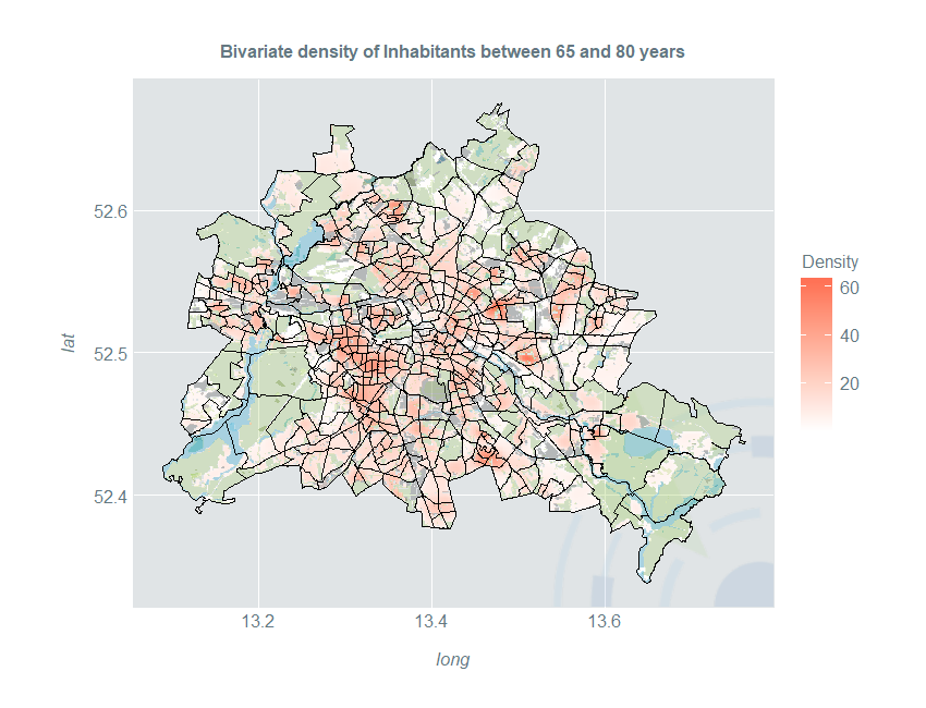
Now we perform the same data preparation steps as in the previous part and estimate the boundary-corrected density of people between 65 and 80 in Berlin. The shapefile of uninhabited areas now goes into the deleteshapes argument:
dataIn <- cbind(do.call(rbind, lapply(berlin@polygons, function(x) x@labpt)),
                  data$E_E65U80)

est <- dshapebivr(data = dataIn,
                  burnin = 5,
                  samples = 15,
                  adaptive = FALSE,
                  shapefile = berlin,
                  deleteShapes = berlinUnInhabitated,
                  gridsize = 325,
                  boundary = TRUE)
To plot the map in ggplot2, we need to perform some additional data preparation steps:
berlin@data$id <- as.character(berlin@data$PLR)
berlinPoints <- fortify(berlin, region = "id")

berlinDf <- left_join(berlinPoints, berlin@data, by = "id")

kData <- data.frame(expand.grid(long = est$Mestimates$eval.points[[1]],
                                lat = est$Mestimates$eval.points[[2]]),
                    Density = est$Mestimates$estimate %>% as.vector) %>%
  filter(Density > 0)
Now, we are able to plot the density together with the administrative districts and uninhabited areas of different types:
ggplot(kData) +
  geom_raster(aes(long, lat, fill = Density)) +
  ggtitle("Bivariate density of Inhabitants between 65 and 80 years") +
  scale_fill_gradientn(colours = c("#FFFFFF", "coral1"))+
  geom_polygon(fill = "grey20", data = fortify(gIntersection(berlin, berlinOther)),
               aes(long, lat, group = group), alpha = 0.25) +
  geom_polygon(fill = "darkolivegreen3", data = fortify(gIntersection(berlin, berlinGreen)),
               aes(long, lat, group = group), alpha = 0.25) +
  geom_polygon(fill = "deepskyblue3", data = fortify(gIntersection(berlin, berlinWater)),
               aes(long, lat, group = group), alpha = 0.25) +
  geom_path(color = "#000000", data = berlinDf, size = 0.1,
            aes(long, lat, group = group)) +
  coord_quickmap()
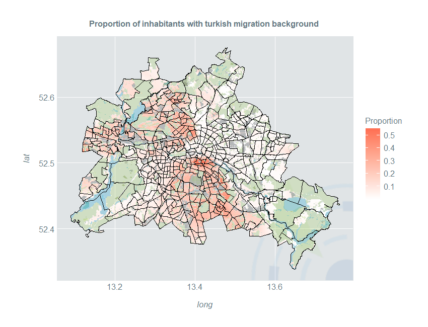
Smooth Estimates of Proportion
One may not only estimate the density, but also the proportion of a certain group relative to the overall population. The Kernelheaping package provides the dshapebivrProp() function which smoothly estimates the spatial proportion using a Nadaraya-Watson-type estimator. Naturally, it includes boundary correction as well. We use another open data example for Berlin on inhabitants with migration background from https://daten.berlin.de/datensaetze/einwohnerinnen-und-einwohner-mit-migrationshintergrund-berlin-lor-planungsräumen
First, we load the dataset and merge the area ids such that they fit with the shapefile of Berlin:
berlinMigration <- read.csv2("EWRMIGRA201512H_Matrix.csv")
berlinMigration$RAUMID <- as.character(berlinMigration$RAUMID)
berlinMigration$RAUMID[nchar(berlinMigration$RAUMID) == 7] <-
  paste0("0", berlinMigration$RAUMID[nchar(berlinMigration$RAUMID) == 7])
berlinMigration <- berlinMigration[order(berlinMigration$RAUMID), ]
We model the spatial proportion of inhabitants with Turkish migration background. For the proportion, a fourth column with the total number of people in that area is necessary:
dataTurk <- cbind(do.call(rbind, lapply(berlin@polygons, function(x) x@labpt)),
                  berlinMigration$HK_Turk,
                  berlinMigration$MH_E)
We estimate the proportion with the dshapebivrProp() function now:
estTurk <- dshapebivrProp(data = dataTurk,
                          burnin = 5,
                          samples = 10,
                          adaptive = FALSE,
                          deleteShapes = berlinUnInhabitated,
                          shapefile = berlin,
                          gridsize = 325,
                          boundary = TRUE,
                          numChains = 4,
                          numThreads = 4)
Now we can plot these proportions:
gridBerlin <- expand.grid(long = estTurk$Mestimates$eval.points[[1]],
                          lat = estTurk$Mestimates$eval.points[[2]])

kDataTurk <- data.frame(gridBerlin,
                        Proportion = estTurk$proportions %>% as.vector) %>%
  filter(Proportion > 0)


ggplot(kDataTurk) +
  geom_raster(aes(long, lat, fill = Proportion)) +
  ggtitle("Proportion of inhabitants with turkish migration background ") +
  scale_fill_gradientn(colours = c("#FFFFFF", "coral1")) +
  geom_polygon(fill = "grey20", data = fortify(gIntersection(berlin, berlinOther)),
               aes(long, lat, group = group), alpha = 0.25) +
  geom_polygon(fill = "darkolivegreen3", data = fortify(gIntersection(berlin, berlinGreen)),
               aes(long, lat, group = group), alpha = 0.25) +
  geom_polygon(fill = "deepskyblue3", data = fortify(gIntersection(berlin, berlinWater)),
               aes(long, lat, group = group), alpha = 0.25) +
  geom_path(color = "#000000", data = berlinDf, size = 0.1,
               aes(long, lat, group = group)) +
  coord_quickmap()
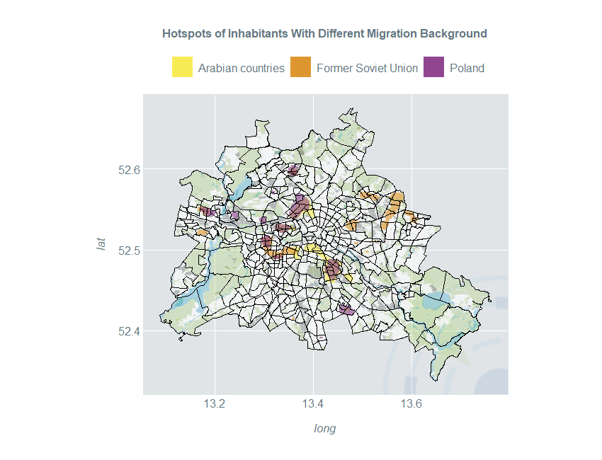
Hotspot Estimation
Spatial kernel density estimates are a great tool to identify subpopulation hotspots. Three different countries / regions of origin are compared: Arabian countries, countries of the former Soviet Union and Poland. We perform the usual data preparation and estimation steps:
dataArab <- cbind(do.call(rbind, lapply(berlin@polygons, function(x) x@labpt)),
                  berlinMigration$HK_Arab)
dataSU <- cbind(do.call(rbind, lapply(berlin@polygons, function(x) x@labpt)),
                berlinMigration$HK_EheSU)
dataPol <- cbind(do.call(rbind, lapply(berlin@polygons, function(x) x@labpt)),
                 berlinMigration$HK_Polen)

estArab <- dshapebivr(data = dataArab, burnin = 5, samples = 10, adaptive = FALSE,
                      shapefile = berlin, gridsize = 325, boundary = TRUE)
estSU <- dshapebivr(data = dataSU, burnin = 5, samples = 10, adaptive = FALSE,
                    shapefile = berlin, gridsize = 325, boundary = TRUE)
estPol <- dshapebivr(data = dataPol, burnin = 5, samples = 10, adaptive = FALSE,
                     shapefile = berlin, gridsize = 325, boundary = TRUE)

gridBerlin <- expand.grid(long = estArab$Mestimates$eval.points[[1]],
                          lat = estArab$Mestimates$eval.points[[2]])
Now we use the 97.5% quantile of the inhabited area to define hotspots:
kDataArab <- data.frame(gridBerlin,
                        Density = estArab$Mestimates$estimate %>% as.vector) %>%
  filter(Density > 0) %>%
  filter(Density > quantile(Density, 0.975)) %>%
  mutate(Density = "Arabian countries")

kDataSU <- data.frame(gridBerlin,
                      Density = estSU$Mestimates$estimate %>% as.vector) %>%
  filter(Density > 0) %>%
  filter(Density > quantile(Density, 0.975)) %>%
  mutate(Density = "Former Soviet Union")

kDataPol <- data.frame(gridBerlin,
                       Density = estPol$Mestimates$estimate %>% as.vector) %>%
  filter(Density > 0) %>%
  filter(Density > quantile(Density, 0.975)) %>%
  mutate(Density = "Poland")
Now, we display the hotspots of all three population subgroups in a single plot:
ggplot() +
  geom_raster(aes(long, lat), fill = "#FFFFFF", data = kData, alpha = 0.6) +
  geom_raster(aes(long, lat, fill = Density), data = kDataArab, alpha = 0.6) +
  geom_raster(aes(long, lat, fill = Density), data = kDataSU, alpha = 0.6) +
  geom_raster(aes(long, lat, fill = Density), data = kDataPol, alpha = 0.6) +
  scale_fill_manual(guide_legend(title = ""), values = c("#f8eb4a", "#DD9123", "#8A3B89")) +
  ggtitle("Hotspots of Inhabitants With Different Migration Background") +
  geom_polygon(fill = "grey20", data = fortify(gIntersection(berlin, berlinOther)),
               aes(long, lat, group = group), alpha = 0.25) +
  geom_polygon(fill = "darkolivegreen3", data = fortify(gIntersection(berlin, berlinGreen)),
               aes(long, lat, group = group), alpha = 0.25) +
  geom_polygon(fill = "deepskyblue3", data = fortify(gIntersection(berlin, berlinWater)),
               aes(long, lat, group = group), alpha = 0.25) +
  geom_path(color = "#000000", data = berlinDf, size = 0.1,
               aes(long, lat, group = group)) +
  coord_quickmap() +
  theme(legend.position = "top")