Introducing the Kernelheaping Package II

In the first part of Introducing the Kernelheaping Package I showed how to compute and plot kernel density estimates on rounded or interval censored data using the Kernelheaping package. Now, let’s make a big leap forward to the 2-dimensional case. Interval censoring can be generalised to rectangles or alternatively even arbitrary shapes. That may include counties, zip codes, electoral districts or administrative districts. Standard area-level mapping methods such as chloropleth maps suffer from very different area sizes or odd area shapes which can greatly distort the visual impression. The Kernelheaping package provides a way to convert these area-level data to a smooth point estimate. For the German capital city of Berlin, for example, there exists an open data initiative, where data on e.g. demographics is publicly available.

We first load a dataset on the Berlin population, which can be downloaded from: https://www.statistik-berlin-brandenburg.de/opendata/EWR201512E_Matrix.csv

library(dplyr)
library(maptools)
library(fields)
library(ggplot2)
library(RColorBrewer)
library(Kernelheaping)
library(rgdal)
library(rgeos)

data <- read.csv2("EWR201512E_Matrix.csv")

This dataset contains the numbers of inhabitants in certain age groups for each administrative districts. Afterwards, we load a shapefile with these administrative districts, available from: https://www.statistik-berlin-brandenburg.de/opendata/RBS_OD_LOR_2015_12.zip

berlin <- readOGR("RBS_OD_LOR_2015_12/RBS_OD_LOR_2015_12.shp")

berlin <- spTransform(berlin, CRS("+proj=longlat +datum=WGS84"))

Now, we form our input data set, which contains the area/polygon centers and the variable of interest, whose density should be calculated. In this case we' like to calculate the spatial density of people between 65 and 80 years of age:

dataIn <- lapply(berlin@polygons, function(x) x@labpt) %>% 
  do.call(rbind, .) %>% 
  cbind(data$E_E65U80)

In the next step we calculate the bivariate kernel density with the “dshapebivr” function (this may take some minutes) using the prepared data and the shape file:

est <- dshapebivr(data = dataIn, burnin = 5, samples = 10, 
                  adaptive = FALSE, shapefile = berlin, 
                  gridsize = 325, boundary = TRUE)

To plot the map with "ggplot2", we need to perform some additional data preparation steps:

berlin@data$id <- as.character(berlin@data$PLR)
berlin@data$E_E65U80 <- data$E_E65U80
berlin@data$E_E65U80density <- berlin@data$E_E65U80 / 
                               (gArea(berlin, byid = TRUE) / 1000000)
berlinPoints <- fortify(berlin, region = "id")
berlinDf <- left_join(berlinPoints, berlin@data, by = "id")

kData <- data.frame(expand.grid(long = est$Mestimates$eval.points[[1]],
                    lat = est$Mestimates$eval.points[[2]]),
                    Density = est$Mestimates$estimate %>% as.vector) %>% 
  filter(Density > 0)

Now, we are able to plot the density together with the administrative districts:

ggplot(kData) +
  geom_raster(aes(long, lat, fill = Density)) + 
  ggtitle("Bivariate density of Inhabitants between 65 and 80 years") +
  scale_fill_gradientn(colours = c("#FFFFFF", "#5c87c2", "#19224e"))+
  geom_path(color = "#000000", data = berlinDf, aes(long, lat, group = group)) +
  coord_quickmap()

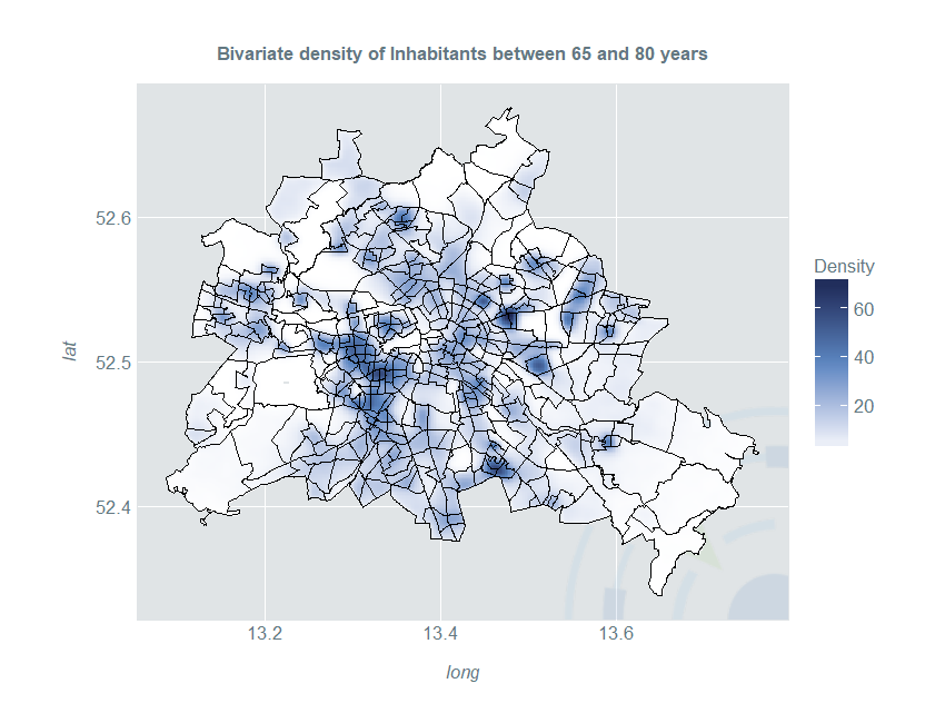
This map gives a much better overall impression of the distribution of older people than a simple choropleth map:

ggplot(berlinDf) +
  geom_polygon(aes(x = long, y = lat, fill = E_E65U80, group = id)) + 
  ggtitle("Number of Inhabitants between 65 and 80 years by district") +
  scale_fill_gradientn(colours = c("#FFFFFF", "#5c87c2", "#19224e"), "n") +
  geom_path(color = "#000000", data = berlinDf, aes(long, lat, group = group)) +
  coord_quickmap()

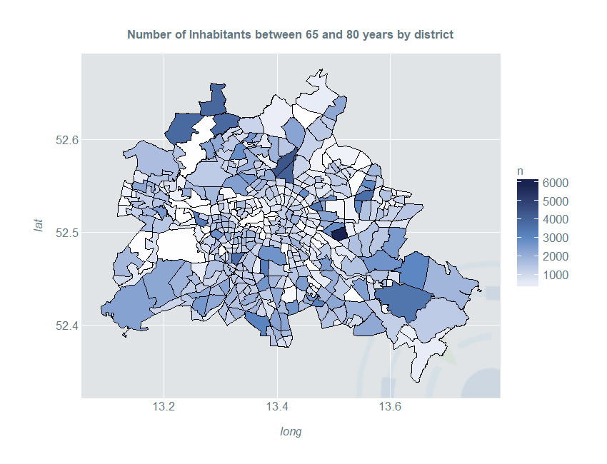
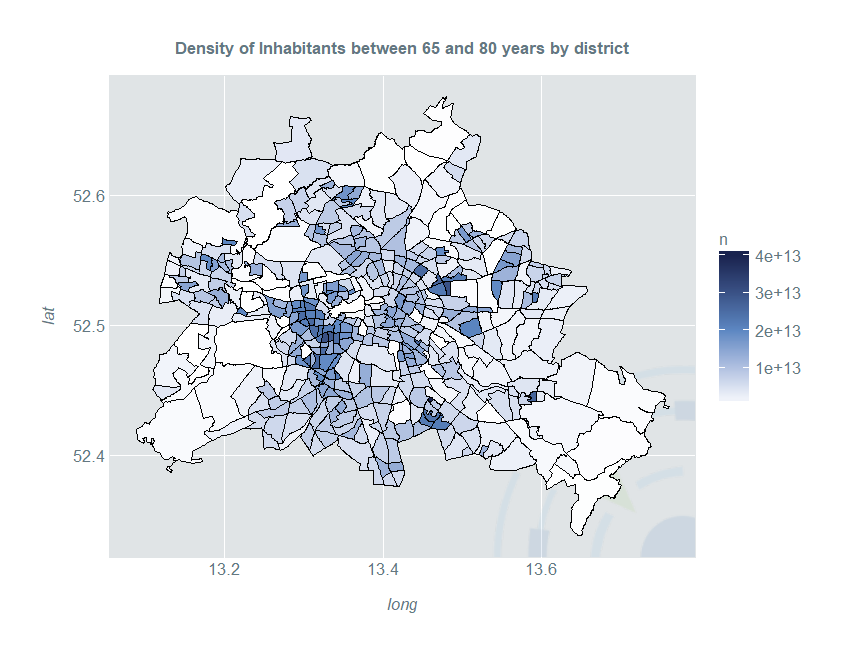
By dividing the count through the area of each shape, we get a density-choropleth-map, which however still suffers from a non-smooth visual impression:

ggplot(berlinDf) +
  geom_polygon(aes(x = long, y = lat, fill = E_E65U80density, group = id)) + 
  ggtitle("Density of Inhabitants between 65 and 80 years by district") +
  scale_fill_gradientn(colours = c("#FFFFFF", "#5c87c2", "#19224e"), "n")+
  geom_path(color = "#000000", data = berlinDf, aes(long, lat, group = group)) +
  coord_quickmap()

Often, as the case with Berlin we may have large uninhabited areas such as woods or lakes. Furthermore, we may like to compute the proportion of older people compared to the overall population in a spatial setting. The third part of this series shows how you can compute boundary corrected and smooth proportion estimates with the Kernelheaping package.