TabPFN: The AI Revolution for Tabular Data
The rapid development of AI models pre-trained on large datasets has greatly simplified the evaluation of unstructured data such as text and images. However, in many core applications in the field of Predictive Analytics (PA), tabular data is still considered. Therefore, the question arises what added value the new AI methods bring to the analysis of tabular data. Will AI also change this area? The capabilities of the new TabPFN method suggest that this is the case. It is a foundation model that was published in the renowned Nature journal in January 2025. On our dataset, which we already used multiple times as a benchmark, it significantly outperforms the algorithm XGBoost in prediction accuracy for small numbers of observations. TabPFN also scores with easily implementable uncertainty quantification. With a larger number of training observations (6000), TabPFN generates a similar prediction accuracy to XGBoost.
The fundamental change in the development of this model compared to algorithms like XGBoost is that the idea of pre-training is transferred to the case of predictions for tabular data. TabPFN was pre-trained on a large number of artificially generated datasets, so the model has inherent knowledge of tabular data out-of-the-box. We will write more about this in the Functionality and Potential of TabPFN section below.
Dataset
Through our partner LOT Internet, we have gained access to a dataset with 8000 data points about vehicles offered on the mobile.de platform. We predict the vehicle price while considering various vehicle characteristics such as mileage, age, and engine power as influencing factors. The application of foundation models for Predictive Analytics has been occupying us for a while. In this blog article, we document how Large Language Models (LLMs) can be used to create tabular predictions. There, we also use free text from the vehicle advertisements in which details about the vehicles are described by the sellers. The dataset used there also contains further tabular features on vehicle equipment.
Results on Car Price Data
In this case, we do not use the free text data because TabPFN cannot process it without major effort. However, categorical features such as the fuel type (diesel, gasoline, etc.) can be included without any problems. The model also takes missing values into account without significant additional effort or loss of observations. There is a Python package for using TabPFN, and instructions can be found in the TabPFN-Github-Repository. The results in Table 1 show that TabPFN brings better performance than XGBoost for 600 observations. The prediction accuracy for 6000 observations, on the other hand, is similarly good. Good predictions can be made very quickly with TabPFN. But the predictions with XGBoost were also made with little time expenditure. We spent about 10 minutes on manual hyperparameter tuning. It should also be noted that we did not perform any feature engineering. It would be interesting to see how this aspect influences the comparison.
| Model | Training Observations | MAPE (%) | Median APE (%) |
|---|---|---|---|
| TabPFN | 600 | 14.2 | 7.3 |
| XGBoost | 600 | 17.3 | 8.5 |
| TabPFN | 6000 | 13.1 | 6.9 |
| XGBoost | 6000 | 13.3 | 7.0 |
Table 1: Results with TabPFN compared to XGBoost on the test dataset of 2000 observations. Number of training observations = 6000. MAPE = Mean absolute percentage error. Median APE = Median absolute percentage error. Features: 9, categorical features: 6.
Prediction Speed
The authors of TabPFN describe it as a potential weakness of the method that the creation of predictions can be slow compared to methods like XGBoost - especially when it comes to a number of observations that is close to 10,000. The method is not suitable for higher numbers of observations. If we use a CPU, the speed disadvantage is confirmed. Our training dataset has 6000 observations with 9 features, while the test dataset has 2000. On a powerful laptop and with a CPU, the prediction took 23 minutes.
In contrast, the prediction on a GPU (tested on an Nvidia L40S) turned out to be very fast - 1.15 seconds for all 2000 observations. So if you have a GPU, the speed disadvantage is no longer so serious. For example, the TabPFN authors state as a reference that a prediction for one observation with the CatBoost algorithm takes 0.0002 seconds. For 2000 observations, that would be 0.4 seconds. Compared to that, TabPFN is about 3 times slower.
Advantage Uncertainty Quantification
The developers of TabPFN write in the Nature paper that the model approximates the Bayesian posterior predictive distribution. A further reference is this paper. As a result, the model outputs a distribution for each observation in the test dataset that quantifies the uncertainty of the prediction. In the code, quantiles of this distribution can be selected that should be output. In this way, it is possible to create 95% uncertainty intervals. In Figure 1, these intervals are shown for our test dataset. This direct possibility of uncertainty quantification is a major advantage over the use of XGBoost and also the use of LLMs to predict a metric target variable. With XGBoost or LLMs, it is not possible to create prediction intervals without additional effort.
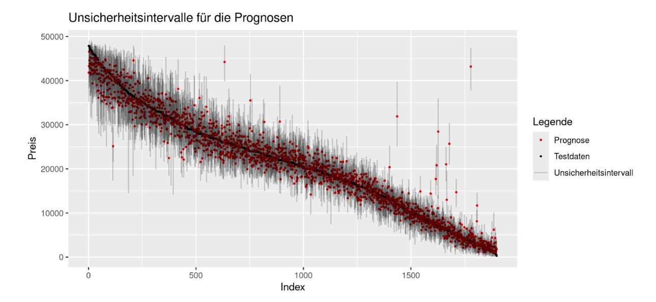
Figure 1: Uncertainty intervals for the predictions on the test data. The values are sorted in descending order from left to right, based on the true prices in the test data.
It turns out that 94.4% of the true test data points lie within the uncertainty intervals of the prediction. This value is very close to the pre-specified value of 95%, which speaks for the quality of the uncertainty quantification.
Functionality and Potential of TabPFN
TabPFN works fundamentally differently than previous state-of-the-art algorithms without pre-training. For pre-training, a large number of artificial datasets were generated. In doing so, as diverse a collection of data as possible was created. This allows the model to learn from examples which functional relationships between features and target variable can occur in tabular data. The approach differs from a traditional approach in which the analyst manually selects a model class that fits the available data. Regarding the potential of the method, the authors of TabPFN make the following assessment:
- The best performance is expected for datasets with up to 10K observations and up to 500 features
- For larger datasets and complex relationships, approaches like CatBoost and XGBoost tend to perform better
- Feature Engineering, Data Cleaning and specialist knowledge of the application area of the method are still necessary to achieve the best prediction results
In addition, the model creates predictions based on entire datasets. As input, it takes the entire training dataset and the test dataset features. The output is the vector of predictions on the test dataset. The authors of TabPFN call this approach In-Context Learning, which differs from XGBoost or even simple models like linear regression in that the latter models create a prediction for each test observation individually after the model has been trained.
In analogy to few-shot learning in LLMs, you can imagine that the training dataset comprises a collection of input-output examples that are passed to the model in the prompt. The model creates predictions for the test data as an answer.
To illustrate what this particularity means with regard to the reproducibility of the results, we examined what happens when we want to make predictions for one fourth of the observations from our test dataset, but this time we do not pass the remaining test observations to TabPFN. With algorithms like XGBoost, this would make no difference because they make a prediction for each observation individually. For TabPFN, however, it turned out that the predictions change. On average, the price predictions differ by €1.50, and at most by €9.10. This is still a weakness of TabPFN. For example, it would be difficult to justify if a customer's creditworthiness were predicted differently depending on which other customers are rated at the same time.
Another disadvantage of TabPFN is that a classic model object cannot be saved, which compresses the learned information from the training data into a small description. For example, a linear model can be described by the estimated coefficients, which requires very little storage space. Another example: The trained XGBoost model object for our benchmark was 3.8 MB in size. In contrast, the saved TabPFN model object required 1.1 GB in our case. In addition, saving the model object saves a lot of time when making further predictions using XGBoost because it does not need to be retrained. Due to the unusual functioning of TabPFN, it does not have this advantage and is currently still relatively slow in generating predictions.
Summary
TabPFN is a very new method for making predictions on tabular data. The functionality is fundamentally different from competing methods. TabPFN has received a lot of attention and has the potential to transform Predictive Analytics. We first tried TabPFN on an example and compared the performance with XGBoost.
In our example, the results from the Nature paper on TabPFN are confirmed. Under certain circumstances, the method enables significantly better prediction accuracy than, for example, XGBoost. This applies especially when the sample size is rather small (in our case with 600 observations). With 6000 observations, TabPFN and XGBoost are close together.
TabPFN did not require any hyperparameter optimization, as we normally do with XGBoost. Another advantage is the simple possibility of creating prediction intervals for the individual observations.
In terms of prediction speed, TabPFN is about a factor of 3 slower than XGBoost, provided that a GPU is available. With a CPU, the speed disadvantage is more serious. Another disadvantage is that a prediction for the same observation can change slightly depending on which other predictions are made simultaneously.
After this first test, we will definitely take a closer look at TabPFN and create further benchmarks.