White Paper: Customer Lifetime Value

The Customer Lifetime Value as the Key Figure for Companies to Guide the Customer Relationship

The Customer Lifetime Value (CLV) is the total worth that a customer generates for a company over their entire customer journey. In many companies, this enormously important figure is used across departments to distribute resources in a way that best optimizes sales and profits. CLV takes into account not only historic and current sales, but also includes forecasted future sales.

Objectives of CLV Analysis

Differentiation of Customers

Which customer is profitable for my company, and which one hurts my bottom line? Answering this interesting question in a data-driven manner is the primary goal of CLV analysis. Not only must one consider past purchase history and the customer’s current behavior, but also their anticipated shopping behavior in the future. It is often the case that customer profitability assumptions are made intuitively; for example, one may assume that those customers that order frequently are also especially profitable. However, this may be far from accurate. The CLV helps to avoid such mistakes, and obtain information based on actual data and facts.

Targeted Control of Customer Relationship Management

As soon as you know which customers are profitable for you, you can adjust your customer relation strategy. Unprofitable customers could, for example, be excluded from a mailing such that those resources can be used more profitably elsewhere. This also allows for more attention for those customers that generate a profit for your company.

Exploit Sales Potential

Service is expensive, yet key for customer satisfaction. Many profitable customers have yet to reach their maximum profitability, and a better understanding of this customer and a higher level of service provision can help to reach that profitability goal. Such a targeted approach can turn service into an effective investment.

Ultimately, this results in double benefits: On the one hand you save by not investing in unprofitable customers, and on the other hand you can use these resources to invest in those that do generate a special profit.

However, challenges also exist with the concrete implementation of CLV. This paper provides an overview of the basics of CLV analysis, and the many possible uses. Current methods and their respective strengths and weaknesses are discussed, as well as strategies for assessing the results of CLV forecasts.

Customer Lifetime Value: What’s Behind It?

A customer lifetime value analysis offers the possibility to quantify the value of a customer in a data-driven manner, quantifying it in a single number. It is ideally suited for assessing and steering various CRM measures, or measures to win new customers. Ironically, many firms are reluctant to use CLV analysis because they find it “too academic”. But, assuming a pragmatic operationalization, the CLV is a rock-solid metric that helps to identify the best customers.

In theory, the CLV covers a large number of potential dimensions, as illustrated in Figure 1. It makes sense that it is challenging for companies to imagine how all of these dimensions are to be captured and calculated to create the CLV. However, measuring every dimension is not necessary at all. The recommendation presented in this paper relies more on a pragmatic conversion on the basis of the order history, which is typically easily accessible. In the context of the “80-20 Rule”, even this minimal effort can result in a large value-add. Of course, the model could also be extended at a later point in time by adding further dimensions. For example, reference potential (the willingness of a customer to recommend), and the value of the newly-recommended customers, could augment the basic model.

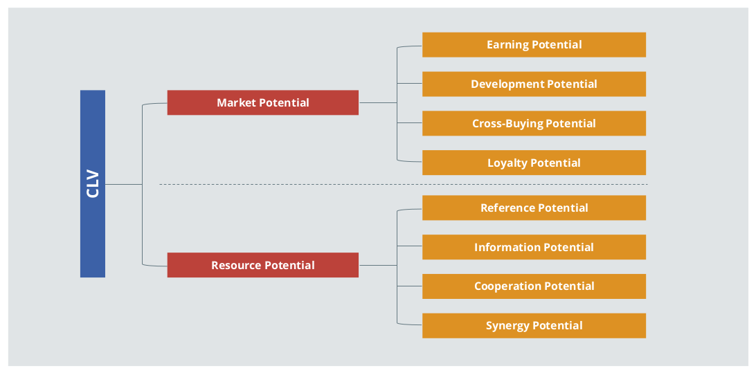Figure 1: Facets of the CLV (Illustration based on Torsten Tomczak / Elisabeth Rudolf-Sipötz (2009): Bestimmungsfaktoren des Kundenwertes: Ergebnisse einer branchenübergreifenden Studie p. 132, in: Bernd Günter/Sabrina Helm: Kundenwert, Grundlagen - Innovative Konzepte - Praktische Umsetzungen, Springer, p. 127-155)

Retrospective vs. Prospective CLV

For existing customers, a distinction is often made between retrospective and prospective customer lifetime value. Retrospective CLV can easily be calculated on the basis of existing data, and falls into the area of internal accounting. Even though this may provide interesting information, it cannot offer a glimpse into the future. Customers change their behavior over time, and it can’t be assumed that findings from a retrospective CLV are well-suited as a forecast. For that, a prospective CLV which uses statistical methods to predict future customer behavior is required. This includes the metrics in a retrospective CLV, but also predicts trends and changes in customer behavior.

Purchase Model vs. Subscription Model

The concrete implementation of a CLV analysis differs based on the business model. With the transaction-oriented purchase model (e.g. car rentals, online fashion retailers), the benefit that a customer will bring to the company over a certain period of time (say, the next 365 days) is of interest. This can be operationalized, for example, by the expected value for contribution margin, turnover, or number of orders in this period. If, on the other hand, the business is subscription-based (e.g. mobile telephones), then the remaining duration of the customer relationship is the primary area of interest. In this case, the goal is to identify whether a customer is acutely at risk of migration, or whether the customer affiliation is very high (given that a high expected affiliation corresponds to a high CLV).

Sales vs. Contribution Margin

If the monetary customer value is calculated, both sales and contribution margins are suitable forecast targets. Sometimes contribution margins are not available in a CRM system, so sales would be used in these cases. If contribution margin data is available, however, this would be the advised forecast target. This is because the contribution margin more accurately reflects the value of the customer for the company, as the costs are already considered. For example, a high turnover can result in a low contribution margin if a customer regularly buys high-priced items on sale. On the other hand, a customer with a moderate turnover can be more valuable if their turnover is comprised of items with a very high contribution margin. If neither sales nor contribution margins are available with reliable accuracy, and the values of the orders or purchased items do not differ very much from one another, it is also possible to rely on the mere number of orders or items.

Customer Lifetime Value: Many Possible Applications

Companies invest large amounts of financial resources in new customer acquisition and customer loyalty management. If these resources are applied incorrectly, this not only results in unnecessary expenses, but in the worst case even the acquisition of unprofitable customers. CLV helps guide resources in a more targeted and profitable way.

For example, when evaluating new customer acquisition measures in online marketing one often only considers the number of new customers a channel delivers. However, this may result in focusing on a channel that delivers many customers, but unprofitable ones. In the worst-case scenario, this approach rewards a dubious affiliate partner that aggressively uses vouchers and delivers customers who may not order, or who order once and end up returning items, for example. A more valuable channel that delivers a few loyal customers may therefore receive less resources. The decisive factor for budget allocation should not be how many new customers are acquired through one channel, but how valuable these customers are. A CLV analysis quantifies this customer value so that the profitability of different channels can be assessed much more accurately, allowing the budget to be invested more sensibly and profitably.

CLV’s potential applications are far from limited to winning the right customers. There are also many possible uses in customer loyalty management: for example, vouchers or free extras can be used to motivate particularly valuable customers to make a purchase or renew a contract. These incentives should be targeted in their application, rather than distributed to all customers according to the “Watering Can Principle.” The challenge is determining how valuable a customer actually is in order to be able to make this determination. CLV can provide a suitable remedy for the problem.

Last but not least, the calculation of the CLV generates insightful information about how different metrics are related to the customer’s value. This makes it possible to check existing assumptions, but also to uncover previously unknown effects from which further CRM measures can often be derived.

Data

The minimum data required for a CLV calculation are the customer’s order history including the number of items, prices, contribution margins, discounts, and return information. These data can also be combined with other customer information such as age, gender, or region. If there are fundamental changes during the analysis period such as a notable increase in sales due to an effective advertising campaign, this information should also be included in the analysis.

Business Model Individualization

CLV can be calculated on the basis of the aforementioned data, for which numerous SaaS solutions are available. However, CLV can only be fully exploited if additional metrics are added that are meaningful for a particular business model. A custom algorithm allows for business-specific data to be analyzed. For example, completely different metrics are relevant for a car rental company than for an online fashion shop, or a telephone provider. Depending on the product or service, these could be characteristics or categories of the products purchased, duration and intensity of use, additional services booked, time of transaction (e.g. day of the week, season), or payment method.

The consideration of such specific metrics makes the CLV calculation not only more accurate, but also offers greater potential for insights into the relationships between metrics and the customer’s value.

Online Tracking Data

Most companies have a large amount of data on the online behavior of their customers at their disposal. The question often arises as to whether this is relevant to the CLV calculation. For businesses with low order frequency, tracking data is a helpful supplement to obtain more high-frequency information. Those with higher order frequency can also benefit from information about additional contacts beyond their orders as well.

However, the usefulness of online tracking data depends on how well these data can be matched with the individual customers. Since customers are often not logged in while on a company website, such feasibility is based on the cookie settings in the customer’s browser. If customers typically access the company website on a tablet or mobile, it is easier to overcome this hurdle since customers are often logged into apps with a username. These checks for quality and plausibility should be done before the analysis to decide whether the use of online tracking data makes sense.

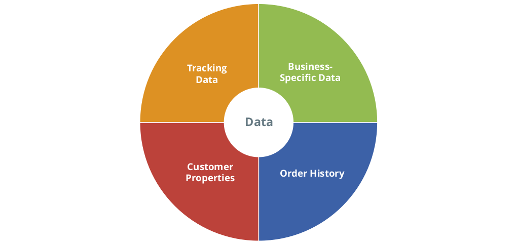Figure 2: Data Usable for CLV Calculation.

Checking the Data Quality

The forecast results can only be as good as the data used in the calculation. Therefore, the quality of all data used should be carefully examined. This includes, for example, checking for deviations from the documentation, missing or inconsistent values, consistency problems, or outliers.

Possible questions include:

• Are there implausible values (e.g. negative length of stay at hotels, very old age)?
• Are test customers or internal accounts still included in the data?
• Do individual customers (e.g. corporate customers) with extremely high turnover appear in the data, distorting the analyses?

Uncovering inconsistencies does not mean that the project is doomed to failure. Rather, it is often sufficient to exclude individual extreme observations (or set them at a less extreme value), limit the analysis period, or, if necessary, exclude individual metrics from the analysis. If these measures fail to remedy the issue, it is better to accept a delay in the project until improved data are available, rather than obtain results that are based on incorrect data.

Selecting the Analysis Period

Despite the fact that the term “CLV” includes the word “lifetime,” the entire customer history does not usually have to be taken into account for the analysis. While the data period must be sufficiently long to achieve a satisfactory forecasting quality, there are even some scenarios where too long of an analysis period is disadvantageous. For example, in some cases, information from orders placed in the distant past can worsen the forecast, as the underlying mechanisms have changed too much over time. This problem can also be taken into account by weighting the data accordingly.

The optimal time period depends on the typical order frequency for the relevant products and services. The length of the required data history depends primarily on the typical customer order frequency. For example, travel bookings may require a longer order history (several years), while grocery orders might need only a few weeks or months.

It may also be useful to consider seasonality when choosing the study period. As a rule, the number of orders varies systematically over the week and over the year, such as during typical vacation periods or the holiday season. To avoid the unwanted influence of these fluctuations on the analysis, it is advisable to always cover the corresponding periods completely in the data (e.g. two years instead of only one and a half).

Lastly, the data should span at least twice as long as the desired forecast period, ideally even longer. To illustrate, this means that to calculate the CLV for one year, for example, at least two years of customer history data should be available.

Statistical Modeling

There are a number of different methods for calculating the CLV which vary in terms of complexity, interpretability, and maintenance requirements. They can roughly be divided into two groups: machine learning methods, and statistical regression approaches. There are also mixed forms or combinations of methods from these two areas.

Machine learning algorithms were developed primarily in computer science for the recognition of categories and patterns. In most cases the algorithm is a “black box,” which does not allow any information to be gained about the causal relationships between the metrics used and the predicted variables. Machine learning procedures are often highly automated, but the “sensibility” of the rules used for classification can often not be checked.

Statistical regression approaches in the context of CLV go far beyond multiple linear regression. Rather, it is the class of generalized additive models that comprises a very flexible and proven spectrum of models. These enable the modeling of relationships between a dependent variable and almost any number of explanatory variables.

Furthermore, techniques are available for variable selection, modeling of nonlinear relationships, and for temporal weighting and balancing of the database. Within the framework of modeling, hypotheses about assumed influencing factors can be tested, and cause and effect relationships identified. Regression approaches thus “open the black box” and enable an understanding of the laws that determine a high or low CLV.

The determination of which procedure is best suited to a specific business model takes place during the development of a tailor-made algorithm. Among other things, the optimal statistical implementation is decided in relation to the specific characteristics of the business, data availability, the planned field of application, and the achievable forecasting quality.

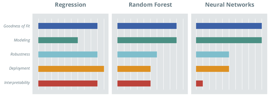Figure 3: Comparison of Selected Statistical and Machine Learning Methods.

Possible Targets and Procedures

At the beginning of each CLV calculation, the target value of the analysis must be selected. Possible targets include:

• Affiliation: Remaining duration of customer relationship (especially with subscription models)
• Purchase likelihood: The probability that a customer will make a purchase within the specified forecast period
• Number of orders: Anticipated number of orders in the forecast period
• Sales or contribution margin: Expected total sales or contribution margin in the forecast period

Depending on the target variable, a variety of methods from the field of regression analysis and machine learning are available for selection. The aim is to select the optimal approach for your specific requirements:

• Random Forest
• Random Survival Forest
• Classification Trees
• Regression Trees
• Support Vector Machines
• Support Vector Regression
• Neural Nets
• Logistic Regression
• Poisson Regression
• Survival Models
• Generalized additive models
• Ridge or Lasso Penalization

Multiple approaches can also be combined to achieve a better result.

Comparison of Procedures

Every statistical approach has strengths and weaknesses. The challenge is choosing the approach that is most appropriate for the situation and business model that delivers the most benefits. To achieve this, the forecast accuracy can be compared for different concrete modeling results. There are also some general characteristics that distinguish different approaches. Figure 3 visualizes the strengths and weaknesses for regression approaches, random forests, and neural nets, for example.

Forecast Quality

A high forecast quality is integral to a good model. In addition to the scope and quality of the data, the model also influences the quality of the forecast. Since machine learning algorithms automatically decide which metrics are used for forecasting and in which form, the information contained in the data is usually used optimally. Therefore, regression approaches can be inferior with regard to forecast quality if ill-considered decisions are made during regression modeling: for example, by excluding metrics without a systematic investigation into the consequences for the predictive quality, or the omission of an important interaction between two metrics. This can be prevented by an exchange with technical experts.

Modeling

Within the framework of modeling, it must be decided which metrics are to be included in the model and in what form (for example, linear or non-linear, individually or as an interaction, etc.). Machine learning algorithms are usually highly automated, so relatively little time has to be invested in the modeling process. With regression approaches, in contrast, each change has to be checked “by hand” for whether or not it improves the model. This is both a strength and weakness: more time and expertise must be invested, but domain-specific knowledge can be purposefully implemented.

Robustness

A pre-requisite for a good forecast is that the model is able to map the variation in the existing data. To have a robust model, it must also be able to produce a stable forecast on the basis of new data in the future. For example, extreme values on individual metrics must not lead to highly distorted, unrealistic forecasts. Methods are available for both regression and machine learning approaches to test and ensure robustness.

Deployment and Maintenance

Once the CLV forecasting model development has been completed, the next step is usually deployment to create the forecasts in real time in the company's internal CRM system. If statistical software is available in the customer back-end, the implementation effort does not differ significantly between the approaches. However, if the forecast is to be implemented in a different programing language (e.g. Java, SQL), this is associated with considerably less effort for regression approaches. In this scenario model coefficients, which can be stored in the form of a mapping table, only have to be inserted into a simple formula, which can easily be done in any language.

Interpretability of the Results

Machine learning algorithms are very often black box approaches that identify the relationships between variables, but whose parameters cannot be interpreted in terms of content (e.g. neural networks) or are very difficult to interpret (e.g. Random Forest). Regression models, on the other hand, have the advantage that the identified cause and effect relationships can be interpreted in the form of directly-interpretable coefficients and the associated information on statistical reliability.

Example: Interpretability of the Results

The following figure illustrates the relationship between the number of support requests and the CLV in a regression model with consideration of nonlinear effects. The relationship is counterintuitive: one would expect support requests to be a sign of dissatisfaction with the product, with the result that the CLV generally decreases as the number of requests increases. In this case, however, the picture is different. In the range from zero to two support requests, the CLV initially increases, and then decreases. This shows that a moderate number of support requests is beneficial for the CLV, in the case of the product under consideration. This product is likely a more complicated product, which many customers are only satisfied with once they’ve received support. From this insight, concrete measures can be taken to increase customer satisfaction, and thus CLV; in the event of initial difficulties, customers should be encouraged to contact support. Also, well-trained support personnel in sufficient numbers can ensure that requests can be processed promptly, resulting in satisfied, loyal customers.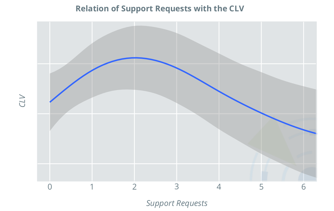

Assessment of Model Quality

Model Adjustment vs. Forecast Quality

During model development, the model is naturally adapted to the underlying data. This means that flexible models inevitably have an advantage during the early stages, because they can easily adapt to the available data. However, the decisive factor is not an optimal adaptation to the already-known data, but rather a reliable forecast for the future. For this reason, it is not the flexible model that should be favored, but rather more robust models that do not adapt to every small (possibly random) irregularity in the data, but rather reflect the fundamental principles.

In order to assess whether a model developed on the basis of known data also provides reliable forecasts, the out-of-sample quality can be considered. For this, the last period in the data (e.g. the last month or year) remains out of the original batch of known data. Data from this period are the “test data”. The model is calibrated on the remaining data (“training data”). Once the model is ready based on the training data, it is asked to forecast over the same period as the test data, and the values are compared. This is a reliable way to estimate the accuracy of the predictions.

Quality Measures

There are a multitude of quality measures for statistical models, depending on the exact model class. One such measure is the R², a figure between 0 and 1 that represents the amount of variation in the actual values can be represented by the model. Other measures include the mean absolute, squared, or percentage deviation of the forecast from the actual values.

Determining which quality measure should be the main focus of the assessment depends, among other things, on the concrete use case. For example, if acquisition costs and customer monetary value are to be compared, it is particularly important that customer values accurately represent the correct average. In this case, a consideration of the deviation would be the most meaningful. In an alternative scenario such as customer relationship management, it is often desired that customers be grouped into categories (A/B/C). For this, it is particularly important that coverage of the forecast categories with the actual categories is as high as possible. The specific CLV values are less relevant in this case than the correct ranking of customers according to their CLV.

When is the Forecast “Good?”

Sometimes it is not easy to judge whether a concrete value for a given measure of quality is "good" or "bad". In order to get an idea of whether the model quality achieved is satisfactory in the context of the available data and metrics, it is therefore advisable to calculate a so-called "zero model" for comparison. This can be a very simple model (e.g. last year's contribution margin as a forecast for the coming year), or a previously used method for CLV calculation. All of the measures of quality considered can then also be calculated for the zero model, and compared with those of the other model. This allows the benefit of evaluating a complex statistical model more precisely.

The required forecast accuracy also depends on the application area of the CLV. For instance, when defining measures that relate to individual customers, sufficiently accurate forecasts are required in order to be able to make a reliable decision in individual cases. If, however, entire cohorts are analyzed - as in the comparison of channels for new customer acquisition - the requirements for forecasting quality are significantly lower.

Further information about the strengths or weaknesses of a model can be obtained by looking at the quality measures differentiated by groups, such as customer groups from a customer segmentation (regions or classified according to the duration of the customer relationship), total sales, or number of orders.

Conclusion

INWT can develop a customized algorithm for predicting the CLV, and identify the optimal modeling approach for the business model and data. The CLV allows one to quantify the value of their customers, which can be used to reliably assess customer acquisition strategies and target customer retention in an effort to retain customers who are at a risk of churning, or who are particularly profitable. In addition to RFM metrics, you can also consider customer characteristics, business model-specific characteristics, and tracking data. In this way, investment in customer acquisition and loyalty management can be much more targeted, and unnecessary investments can be avoided.

As a result, you not only receive the calculated CLV at the time of project execution, but also the tools to calculate the CLV in real time in the future, including new customers, on the basis of updated data in your CRM system.