Who’s best in class? Comparing forecasting models with a Predictive Analytics Cube (PAC)
The problem of (comparable) forecasting
Over the last years, time series forecasting has become a subfield of Data Science where well established statistical and econometric methods mingle with modern ML techniques. However, solid standards with regard to data partitioning or comparable model evaluation have not been established yet.
Forecasting is central to our work at INWT. We use it for a wide range of applications including predicting sales, staff planning and air quality monitoring. When announcements of shiny, new forecasting methods pop up in our timelines, we are faced with the challenge to separate the wheat from the chaff - does this new method really deliver on its promises? Or rather, does it deliver when applied practically in a controlled environment and on data chosen by us? What exactly are the strengths and weaknesses of this particular forecasting method? To answer these questions, we decided to build our own Predictive Analytics Cube (PAC).
The purpose of our PAC is to build an infrastructure of data, methods, predictions and reports that allows fast comparison of methods regarding their predictive power based on standardized evaluation. We want our PAC to help us make quick and better informed model class selection decisions when faced with a specific forecasting problem. Which method looks most promising for instance, for a low frequency time series with strong seasonality and trend? And when a new method enters the forecasting arena: how well does it perform on a well known dataset, and how does it compare to other methods? We want our PAC to give us a legitimate and sophisticated answer to the question “Which method is best in class?”. And if the answer turns out to be ambiguous, that’s fine.
We decided to build our own PAC, to have a tailored solution to our goals at INWT and to be able to deliver high quality, state-of-the-art solutions to our customers. We want to be able to extend it easily with new methods and data. Hence we chose not to fork similar projects, like the impressive Monash Time Series Forecasting Repository or the innovative Out-of-sample time series forecasting package, but take these projects as inspiration and guidance.
Building our own PAC
In our first, minimal version of the PAC we include four models and three univariate time series. As of now, we limit the PAC to univariate forecasting and future values are exclusively predicted using the past values of a time series. Let’s take a look under the hood of the cube to see how we wove the data, methods and reports together.
Architecture
Two R packages that we developed build the backbone of our PAC. PacModel queries the training data from a MariaDB database and hands it over to the models. Models run on the training data and send their insample predictions as well as their out of sample predictions back to the database. PacReport then queries these forecasts and produces an extensive html report via rmarkdown.
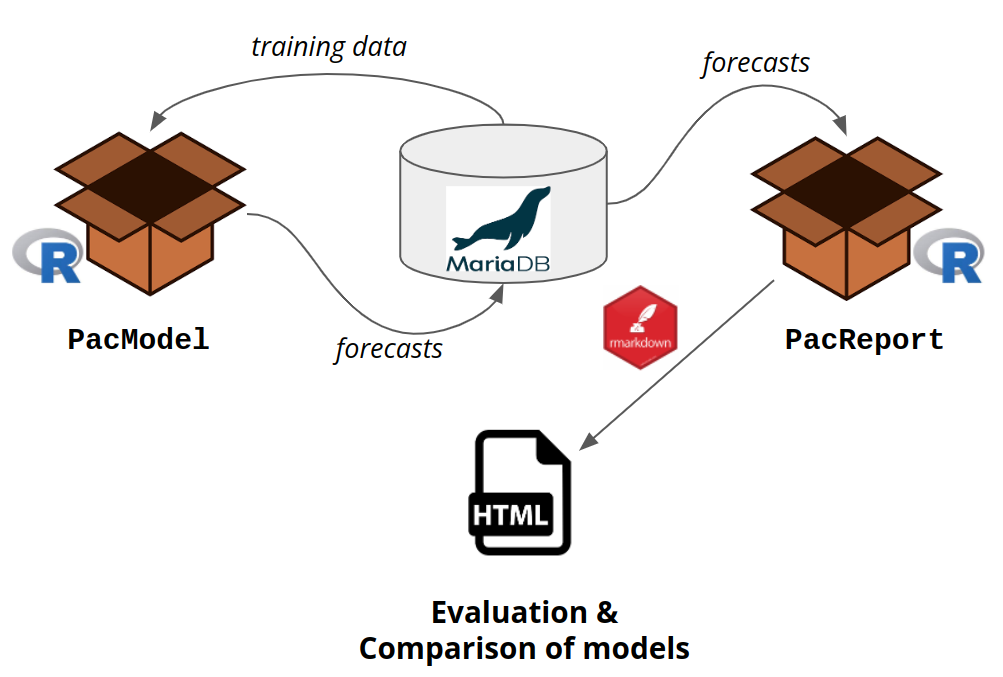 Current PAC architecture
Datasets
| Time Series | Info | Observations (Frequency) | Source |
|---|---|---|---|
| Real gross domestic product (GDP) of Germany in price-adjusted million euros (base year 2010) | Not seasonally adjusted. 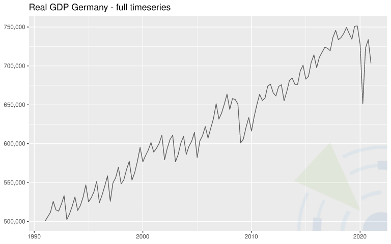 | 121 (quarterly) | Eurostat, Real Gross Domestic Product for Germany CLVMNACNSAB1GQDE, retrieved from FRED, Federal Reserve Bank of St. Louis. |
| Electricity Demand in New South Wales (NSW) Australia | Data was aggregated on a daily level. 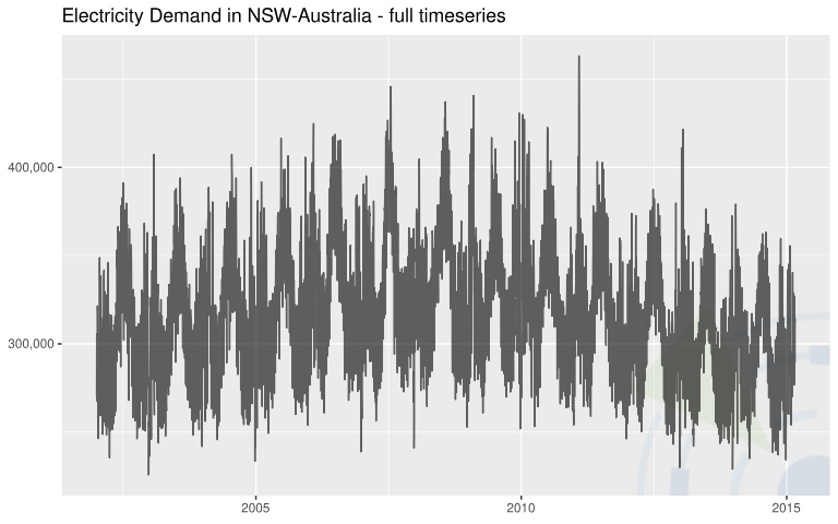 | 4807 (daily) | Godahewa, Rakshitha, Bergmeir, Christoph, Webb, Geoff, Hyndman, Rob, & Montero-Manso, Pablo. (2021). Australian Electricity Demand Dataset (Version 1) Data set. Zenodo. |
| Solar power production in Megawatts (MW) in Australia | Data was aggregated on a daily level to remove the zero-value periods at night. 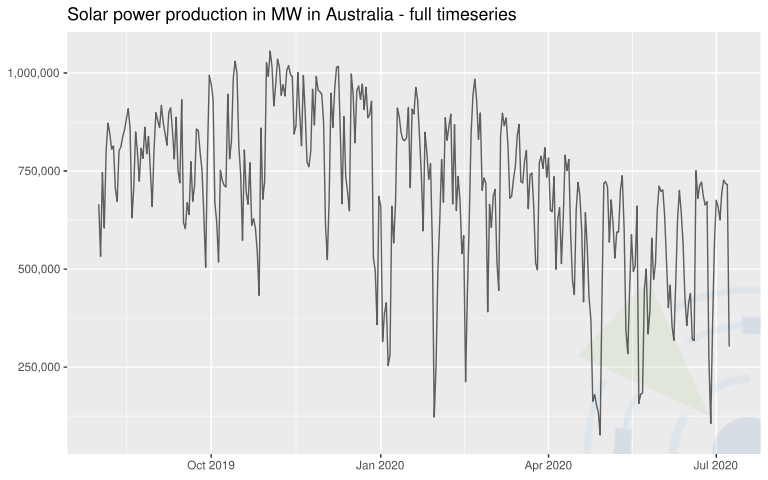 | 343 (daily) | Godahewa, Rakshitha, Bergmeir, Christoph, Webb, Geoff, Abolghasemi, Mahdi, Hyndman, Rob, & Montero-Manso, Pablo. (2020). Solar Power Dataset (4 Seconds Observations) (Version 2) Data set. Zenodo. |
Models
| Model | R Package::Function | Info |
|---|---|---|
| ARIMA | forecast::auto.arima() | The function uses a variation of the Hyndman-Khandakar algorithm, which combines unit root tests, minimisation of the AIC and MLE to obtain an (seasonal) ARIMA model. |
| ARIMA W/ XGBOOST ERRORS | forecast::auto.arima() and xgboost::xgb.train() | Like the previous ARIMA model, but additionally uses boosting to improve residuals on exogenous regressors. |
| ETS | forecast::ets() | An exponential smoothing state space model that is similar to ARIMA models in that a prediction is a weighted sum of past observations, but the model explicitly uses an exponentially decreasing weight for past observations. Potential trend or seasonality are estimated automatically, as well as the error, trend and season type. |
Evaluation
We evaluate our models primarily on the basis of their out of sample (oos) performance. To divide the data into training and test data, we chose a rolling origin setup, in which the “size of the forecast horizon is fixed, but the forecast origin changes over the time series [...], thus effectively creating multiple test periods for evaluation.” (Hewamalage et al. 2022) Furthermore, we decided to increase the training data window by one more datapoint with every model run. This approach is also called time series cross-validation (tsCV) (Hyndman, R.J., Athanasopoulos, G., 2021) - a temporal order preserving version of cross-validation. For now, we limit ourselves to 1-step-ahead predictions, but plan to implement flexible forecast horizons in the future.
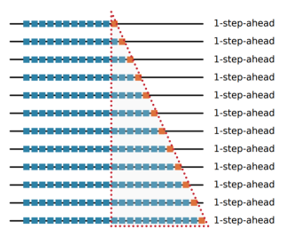 An expanding window, rolling origin oos setup. Blue dots represent training data points, red dots represent test data. Picture taken from Hewamalage et al. 2022.
In order to detect potential problems with overfitting, we additionally measure in sample performance for each model and dataset. To this end, we snapshot the smallest training data window and the biggest training data window for each dataset and evaluate the predictions for these data points. This expanding window, rolling origin oos structure combined with our overfit monitoring provides us with a realistic setup that fits our usual business cases: Available input data increases over time while frequent model recalibration for optimal forecasting performance is both desirable and viable.
To achieve our goal of easy compatibility between methods, we decided to use one method across all datasets as a baseline: an exponential smoothing state space model (ETS). This model delivers pretty good “rule of thumb” forecasts - without any tuning effort at all as the methodology is fully automatic. Our ETS model considers a potential trend or seasonality and conveniently chooses error, trend and season type automatically (either additive or multiplicative). We chose it as our baseline because of its relative simplicity and good “out of the box” performance.
For high level judgments about the predictive power of our different PAC forecasting models, we primarily use relative measures, i.e. ratios of some error measure for the forecasting model divided by that of our ETS benchmark model. Eligible relative measures are for example the Relative Mean Absolute Error (RelMae) or the Relative Root Mean Squared Error (RelRMSE). These relative measures are awesome for being easily interpretable (ratios < 1 stand for a model performance better than baseline on that error measure, > 1 for worse performance) while being conveniently scaled by the benchmark errors on a series level. In other words: For a given dataset, relative measures provide performance statistics comparable across all sorts of models. We are aware of the problems relative measures may cause when presented with a series containing trend or unit root (Hewamalage et al. 2022, pp.44). Luckily, these problems mainly become relevant for longer forecast horizons, which we don’t use at the moment. We decided therefore to postpone tackling them until we actually extend our PAC beyond one step ahead predictions. Also, when examining and testing a specific model of our PAC in-depth, we understand that using multiple evaluation measures is needed and looking at relative measures alone won’t do the job.
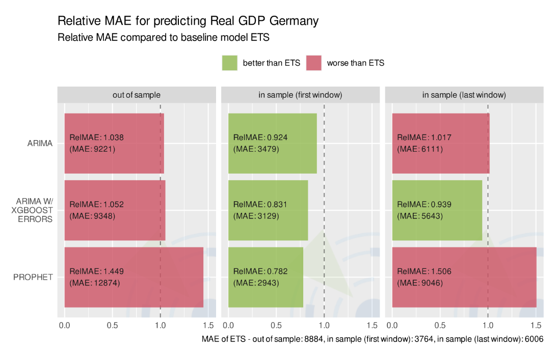 Model performance on predicting time series Real GDP Germany, measured by Relative MAE
Lessons learned and tasks ahead
Our PAC is still in its early stages - it may be considered a minimal viable product. Yet it already provides an easily extendable framework to compare forecasting model performance across different datasets. Even to reach this stage entailed quite a few challenges. One challenge we certainly underestimated is the tradeoff between automation and fine tuning. On the one hand, we want to see how a model works “out of the box” with as little configuration as possible when confronted with different data scenarios. On the other hand, we might not treat a model fairly when knowingly running it with too little configuration. In fact, putting a model in production with very little configuration and fine tuning is not a realistic business scenario for us. Models get fine tuned before they are deployed - but we want our PAC to provide a realistic hint beforehand to what a model’s forecasting capability is.
Another point of discussion when designing our PAC was to find a sensible baseline model that would work across several different time series. This choice is not trivial if you want the baseline to be somewhat naive and flexible to handle seasonality, trend and unit roots at the same time. Within our four initial PAC models, ETS seemed to be the most naive yet sufficiently flexible to qualify as a benchmark. So after a long discussion we opted for ETS as a benchmark knowing that, as the PAC grows, we might have to revise our decision later.
Our project board is full of ideas on how to extend and enhance our PAC from here on. These are a few possible extensions we’re currently considering:
- incorporate exogenous time varying variables which may affect the target series,
- make forecast horizons flexible to allow for n-step-ahead predictions,
- integrate Python models into our otherwise R package supported architecture,
- introduce CI/CD automation (via Jenkins) to carry out a rerun of models and reports when a new model or a new dataset was added to the PAC,
- turn our standardized html report into a vue.js dashboard,
- add new models and datasets.
In any case, this is just the beginning of our PAC. Stay tuned for in-depth analysis of new models and other insights into comparable forecasting.