Code performance in R: Which part of the code is slow?

This is the first part of our series about code performance in R.

Let's assume you have written some code, it's working, it computes the results you need, but it is really slow. If you don't want to get slowed down in your work, you have no other choice than improving the code's performance. But how to start? The best approach is to find out where to start optimizing.

It is not always obvious which part of the code makes it so slow, or which of multiple alternatives is fastest. There is the risk to spending a lot of time optimizing the wrong part of the code. Fortunately, there are ways to systematically test how long a computation takes. An easy way is the function system.time. Just wrap your code into this function, and you will (in addition to the actual results of that code) get the time your code took to run.

Let's draw a lot of random numbers as an example:

system.time(runif(n = 1000000))

##      user      system       elapsed 
##      0.024     0.003        0.027 

The value for user shows the "time charged for the execution of user instructions of the calling process" (see ?proc.time).

system.time is only useful for computations that take a bit longer (at least some seconds). If a single execution takes only microseconds, the result of system.time will vary widely due to tiny tasks your system happens to be doing in the background. It would then be better to run the code several times and look at the mean or median of the computation times. Luckily, the microbenchmark package already provides a tool for this. In addition, you can compare different pieces of code. microbenchmark runs an expression several times (100 times per default) and computes some summary statistics for the computation times. Let's try it out in order to compare two different ways of subsetting:

library(microbenchmark)

microbenchmark(
   "dollarSign" = iris$Sepal.Length[10],
   "brackets" = iris[10, "Sepal.Length"]
)

## Unit: nanoseconds
## expr       min    lq     mean median     uq   max neval
## dollarSign 584   651  1036.28  906.5 1042.5 15651   100
## brackets   8391 9054 11322.02 9355.0 9885.0 49936   100

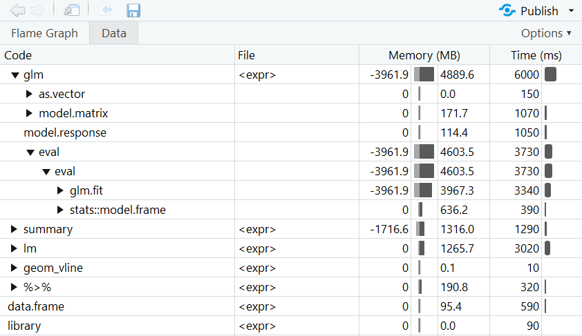
Although both versions lead to the same result, the bracket version clearly took longer on average. But a look at min and max reveals that a single try could have led to a different result! Optimizing a whole script by spending hours with adding system.time or microbenchmark to every single function may sound a bit ineffective to you. A better way would be to use the profiler from the profvis package in RStudio. Just wrap your code into profvis() and run it. The profiler interface will open and give you a very clear overview of which part of the code takes how much time. In the following example, we simulate some data, create two plots, and compute a statistical model twice using two different functions.

library(profvis)

profvis({
  library(dplyr)
  library(ggplot2)
  
  # Simulate data
  n <- 5000000
  dat <- data.frame(norm = rnorm(n),
                    unif = runif(n),
                    poisson = rpois(n, lambda = 5))
  
  # Compute more variables
  dat <- dat %>%
    mutate(var1 = norm + unif,
           var2 = poisson - unif + min(poisson - unif),
           var3 = 3 * unif - 0.5 * norm)
  
  # Plots
  ggplot(dat, aes(x = var1, y = var3)) +
    geom_point() +
    geom_smooth(method = lm)
  ggplot(dat, aes(var1)) +
    geom_histogram() +
    geom_vline(xintercept = 0, color = "red")
  
  # Models
  modLm <- lm(var1 ~ var2 + var3, data = dat)
  summary(modLm)
  modGlm <- glm(var1 ~ var2 + var3, data = dat,
                family = gaussian(link = "identity"))
  summary(modGlm)
})

Note: The computation times always fluctuate due to random influences. This means that the results of system.time, microbenchmark, and the profiler will vary a bit with each execution.